Unit - V: Tests of significance

Unit - V: Tests of significance 

Significance refers to generalization to the population from sample statistics. When sample statistics are close to population statistics or the parameters, generalization becomes easy.
The central limit theorem tells us that, if our sample is large, the sampling distribution of the mean will be approximately normally distributed irrespective of the shape of the population distribution. Before use of statistical tools, it is important to estimate to what extent the data represent all the assumptions of specific tools. Below are some of the assumptions of repeatedly used bi-variate statistics for mean differences.

1. t-ratio

1.1. Testing for Normality

1.2 Homogeneity of variance (homoscedasticity) is an important assumption shared by many parametric statistical methods. This assumption requires that the variance within each population be equal for all populations (two or more, depending on the method). For example, this assumption is used in the two-sample t-test and ANOVA. If the variances are not homogeneous, they are said to be heterogeneous. If this is the case, we say that the underlying populations, or random variables, are heteroscedastic (sometimes spelled as heteroskedastic).(ref: http://link.springer.com/referenceworkentry/10.1007%2F978-3-642-04898-2_590)

2. F-ratio








 t-test, Z-test and F-tests are used  for assessing tests of significance in mean differences when distribution follows normality assumptions. 




All parametric tests assume that the populations have specific characteristics and that samples are drawn under certain conditions. These characteristics and conditions are expressed in the assumptions of the tests.
Ref:http://www.psychology.emory.edu/clinical/bliwise/Tutorials/TOM/meanstests/assump.htm

One-Sample Z Test

The assumptions of the one-sample Z test focus on sampling, measurement, and distribution. The assumptions are listed below. One-sample Z tests are considered "robust" for violations of normal distribution. This means that the assumption can be violated without serious error being introduced into the test. The central limit theorem tells us that, if our sample is large, the sampling distribution of the mean will be approximately normally distributed irrespective of the shape of the population distribution. Knowing that the sampling distribution is normally distributed is what makes the one-sample Z test robust for violations of the assumption of normal distribution.

Interval or ratio scale of measurement (approximately interval)

Random sampling from a defined population

Characteristic is normally distributed in the population

One-Sample t Test

The assumptions of the one-sample t-test are identical to those of the one-sample Z test. The assumptions are listed below. One-sample t-tests are considered "robust" for violations of normal distribution. This means that the assumption can be violated without serious error being introduced into the test.

Interval or ratio scale of measurement (approximately interval)

Random sampling from a defined population

Characteristic is normally distributed in the population

t-Test for Dependent Means

The assumptions of the t-test for dependent means focus on sampling, research design, measurement, and distribution. The assumptions are listed below. The t-test for dependent means is considered typically "robust" for violations of normal distribution. This means that the assumption can be violated without serious error being introduced into the test in most circumstance. However, if we are conducting a one-tailed test and the data are highly skewed, this will cause a lot of error to be introduced into our calculation of difference scores which will bias the results of the test. In this circumstance, a nonparametric test should be used.

Interval or ratio scale of measurement (approximately interval)

Random sampling from a defined population

Samples or sets of data used to produce the difference scores are linked in the population through repeated measurement, natural association, or matching

Scores are normally distributed in the population; difference scores are normally distributed

t-Test for Independent Means

The assumptions of the t-test for independent means focus on sampling, research design, measurement, population distributions and population variance. The assumptions are listed below. The t-test for independent means is considered typically "robust" for violations of normal distribution. This means that the assumption can be violated without serious error being introduced into the test in most circumstance. However, if we are conducting a one-tailed test and the data are highly skewed, this will cause a lot of error to be introduced into our test and a nonparametric test should be used. The t-test for independent means is not robust for violations of equal variance. Remember that the shape of the sampling distribution is determined by the population variance (s₂) and the sample size. If the population variances are not equal, then when we calculate the difference between sample means, we do not have a sampling distribution with an expectable shape and cannot calculate an accurate critical value of the t distribution. This is a serious problem for our test. Our alternatives when the asssumption of equal variances has been violated are to use a correction (available in the SPSS program) or to use a nonparametric test. How do we determine whether this assumption has been violated? Conduct a Levene's test (using SPSS).

Interval or ratio scale of measurement (approximately interval)

Random sampling from a defined population

Samples are independent; no overlap between group members

Scores are normally distributed in the population

Population variances are equal

Data types that can be analysed with z-tests

 data points should be independent from each other
 z-test is preferable when n is greater than 30.
 the distributions should be normal if n is low, if however n>30 the distribution of the data does not have to be normal
 the variances of the samples should be the same (F-test)
 all individuals must be selected at random from the population
 all individuals must have equal chance of being selected
 sample sizes should be as equal as possible but some differences are allowed

---

Data types that can be analysed with t-tests

 data sets should be independent from each other except in the case of the paired-sample t-test
 where n<30 the t-tests should be used
 the distributions should be normal for the equal and unequal variance t-test (K-S test or Shapiro-Wilke)
 the variances of the samples should be the same (F-test) for the equal variance t-test
 all individuals must be selected at random from the population
 all individuals must have equal chance of being selected
 sample sizes should be as equal as possible but some differences are allowed

---

Limitations of the tests

if you do not find a significant difference in your data, you cannot say that the samples are the same

---

Introduction to the z and t-tests

Z-test and t-test are basically the same; they compare between two means to suggest whether both samples come from the same population. There are however variations on the theme for the t-test. If you have a sample and wish to compare it with a known mean (e.g. national average) the single sample t-test is available. If both of your samples are not independent of each other and have some factor in common, i.e. geographical location or before/after treatment, the paired sample t-test can be applied. There are also two variations on the two sample t-test, the first uses samples that do not have equal variances and the second uses samples whose variances are equal.

It is well publicised that female students are currently doing better then male students! It could be speculated that this is due to brain size differences? To assess differences between a set of male students' brains and female students' brains a z or t-test could be used. This is an important issue (as I'm sure you'll realise lads) and we should use substantial numbers of measurements. Several universities and colleges are visited and a set of male brain volumes and a set of female brain volumes are gathered (I leave it to your imagination how the brain sizes are obtained!).

---

Hypotheses

---

Data arrangement

Excel can apply the z or t-tests to data arranged in rows or in columns, but the statistical packages nearly always use columns and are required side by side.

---

Results and interpretation

Degrees of freedom:

For the z-test degrees of freedom are not required since z-scores of 1.96 and 2.58 are used for 5% and 1% respectively.
For unequal and equal variance t-tests = (n₁ + n₂) - 2
For paired sample t-test = number of pairs - 1

The output from the z and t-tests are always similar and there are several values you need to look for:

You can check that the program has used the right data by making sure that the means (1.81 and 1.66 for the t-test), number of observations (32, 32) and degrees of freedom (62) are correct. The information you then need to use in order to reject or accept your H_O, are the bottom five values. The t Stat value is the calculated value relating to your data. This must be compared with the two t Critical values depending on whether you have decided on a one or two-tail test (do not confuse these terms with the one or two-way ANOVA). If the calculated value exceeds the critical values the H_O must be rejected at the level of confidence you selected before the test was executed. Both the one and two-tailed results confirm that the H_O must be rejected and the H_A accepted.

We can also use the P(T<=t) values to ascertain the precise probability rather than the one specified beforehand. For the results of the t-test above the probability of the differences occurring by chance for the one-tail test are 2.3x10^-9 (from 2.3E-11 x 100). All the above P-values denote very high significant differences.

Unit 4: Hypothesis testing

Unit - IV: Hypothesis testing: Formulation and types; null hypothesis, alternate hypothesis, type I

and type II errors, level of significance, power of the test, p-value. Concept of standard error and

confidence interval.

Hypothesis is a conjectural statement of the relation between two or more variables. For example, a study designed to look at the relationship between anxiety and test performance might have a hypothesis that states, "This study is designed to assess the hypothesis that anxious people will perform worse on a test than individuals who are not anxious." 

Hypothesis are always in declarative sentence form, and they relate, either generally or specifically, variables to variables. There are two criteria for "good" hypothesis and hypothesis statements. One, hypothesis are statements about the relations between variables. For example, over-learning leads to performance decrement. Second criterion is that hypothesis carry clear implications for testing the stated relations. For example, groups A and B will differ on some characteristics. So hypothesis can be tested and shown to be probably true or probably false. 

Hypothesis has some virtue. It directs investigation. There are important differences between problem and hypothesis. The problem is a question and is not directly testable. But hypothesis is testable. 

Sources of hypothesis
Hypothesis can be deduced from theory and from other hypotheses. 

Hpothesis testing -

Step1: Make a hypothesis and select a criteria for the decsion The standard logic that underlies hypothesis testing is that there are always (at least) two hypotheses: the null hypothesis and the alternative hypothesis.
The null hypothesis (H₀) predicts that the independent variable (treatment) has no effect on the dependent variable for the population.
The alternative hypothesis (H₁) predicts that the independent variable will have an effect on the dependent variable for the population - we'll talk more about how specific this hypothesis may be
The logic of hypothesis testing assumes that we are trying to reject the null hypothesis, not that we are trying to prove the alternative hypothesis.
Why? Generally, It is easier to show that something isn't true, than to prove that it is. This is especially true when we are dealing with samples. Remember that we aren't testing every individual in the population, only a sub set.
Example :
Hypothesis: All dogs have 4 legs.
To reject: need to have a sample which includes 1 or more dogs with more or fewer than 4 legs. 
To accept: need to examine every dog in the population and count their legs. So part of the first step is to set up your null hypothesis and your alternative hypothesis. The other part of this step is to decide what criteria that you are going to use to either reject or fail to reject (not accept) the null hypothesis. So consider the problem that we have. We have a sample and its descriptive statistics are different from the population's parameters (which may be based on the control group sample statistics). How do we decide whether the difference that we see is due to a "real" difference (which reflects a difference between two populations) or is due to sampling error? To deal with this problem the researcher must set a criteria in advance. For example, think of the kinds of questions we were asking in the previous chapter. Given a population X with a m = 65 and a s = 10, what is the probability that our sample (of size n) will have a mean of 80? We're going to be asking the same questions here, but taking it a step further and say things like, "Gee, the probability that my sample has a mean of 80 is 0.0002. That's pretty small. I'll bet that my sample isn't really from this population, but is instead from another population." setting a criteria in advance is concerned with this part about saying "that's pretty small". When we set the criteria in advance, we are essentially saying, how small a chance is small enough to reject the null hypothesis. Or in other words, how big a difference do I need to have to reject the null hypothesis. That's the big picture of setting the criteria, now let's look at the details:
what are the possible real world situations?
- H₀ is correct
- H₀ is wrong
what are the possible conclusions?
- H₀ is correct
- H₀ is wrong
So this sets up four possibilities (2 * 2):
- 2 ways of making mistakes
- 2 chances to be correct

	Actual situation
Experimenter's Conclusions	H0 is correct H0 is wrong Reject H0 Fail to reject H0 oops! Type I error Yay! correct Yay! correct oops! Type II error the two kinds of error each have their own name, because they really are reflecting different things -type I error (a, alpha) - the H0 is actually correct, but the experimenter rejected it

- e.g., there really is only one population, even though the probability of getting a sample was really small, you just got one of those rare samples
-type II error (b, beta)- the H₀ is really wrong, but the experiment didn't feel as though they could reject it
- e.g., your sample really does come from another population, but your sample mean is too close to the original population mean that you aren't can't rule out the possibility that there is only one population




The courtroom/jury analogy



	Actual situation
Jury's Verdict	X is innocent X is guilty Guilty Not Guilty oops! Type I error Yay! correct Yay! correct oops! Type II error

Type I error - sending an innocent person to jail
Type II error - letting a guilty person go free


In scientific research, we typically take a conservative approach, and set our criterIa such that we try to minimize the chance of making a Type I error (concluding that there is an effect of something when there really isn't). In other words, scientists focus on setting an acceptable alpha level (a), or level of significance.
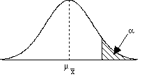
The alpha level (a), or level of significance, is a probability value that defines the very unlikely sample outcomes when the null hypothesis is true. Whenever an experiment produces very unlikely data (as defined by alpha), we will reject the null hypothesis. Thus, the alpha level also defines the probability of a Type I error - that is, the probability of rejecting H₀ when it is actually true.

Let's look at this with pictures of distributions to try and connect this with what we've been talking about so far.
Consider the following sample mean distributions.


	a = prob of making a type I error
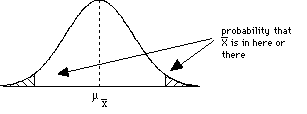
	general alternative hypothesis H0: no difference H1: there is a difference Two-tailed test a = 0.05 so this is 0.025 in each tail 0.025 + 0.025 = 0.05
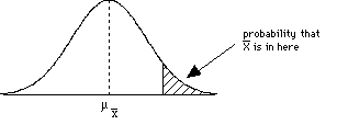
	specific alternative hypothesis H0: no difference H1: there is a difference & the new group should have a higher meanOne-tailed test a = 0.05 so this is 0.05 in the tail

so how do we interpret these graphs?

If our sample mean falls into the shaded areas then we reject the H₀. On the other hand, if our sample mean falls outside of the shaded areas, then we may not reject the H₀. These shaded regions are called the critical regions.
The critical region is composed of extreme sample values that are very unlikely to be obtained if the null hypothesis is true. The size of the critical region is determined by the alpha level. Sample data that fall in the critical region will warrant the rejection of the null hypothesis.

Okay now lets make things concrete with an example:

Population distribution	So the population m = 65 and s = 10. Suppose that you take a sample of n = 25, give them the treatment and get a  = 69.Did the treatment work? Does it affect the population of individuals? Which distribution should you look at? population? sample means?
distribution of sample means	Look at distribution of sample means.Find your sample mean in the distribution. Look up the probability of getting that mean or higher for the sample (see last chapter). Let's assume an a = 0.05 Let's also assume that our alternative hypothesis is that the treatment should improve performance (make the mean higher) now we need to find our standard error.  =  = 10/5 = 2
	what is our critical region? Well, this is a one tailed test. so, look at the unit normal table, and find the area that corresponds to a = 0.05 z = 1.65 (conservative, really 1.645) so, translate this into a sample mean = Z + m = (1.65)(2)+65 = 68.3 so, if = 69, then we reject the H0

Another way that we could have done this question is just to use z-scores.


since we know that the z-score corresponding to the critical region is 1.65, then we just need to compute the z-score corresponding to the sample mean to see if it is higher or lower than this critical z-score.
Z =  = (69 - 65) / 2 = 2.0 since > Z_critical, then we can reject the H₀

For the example that we just did, we made a hypothesis that the treatment would make a difference in a specific direction (ie. treatment would increase the mean).However, the most common way to do hypothesis testing is to make a more general hypothesis, that the treatment will change the mean, either increase or decrease.


Population distribution	So the population m = 65 and s = 10. Suppose that you take a sample of n = 25, give them the treatment and get a  = 69. Did the treatment work? Does it affect the population of individuals?Which distribution should you look at? population? sample means?
distribution of sample means	Look at distribution of sample means.Find your sample mean in the distribution. Look up the probability of getting that mean or higher for the sample (see last chapter). Let's assume an a = 0.05 Let's also assume that our alternative hypothesis is that the treatment should change performance, so we have a two-tailed test.
	now we need to find our standard error.  =  = 10/(sqroot 25) = 2what is our critical region? Well, this is a two tailed test. so, look at the unit normal table, and find the area that corresponds to a = 0.05 z = 1.96 so, translate this into a sample mean  = Z  + m = (1.96)(2)+65 = 68.9 so, if  = 69, then we reject the H0

Assumptions of hypotheses testing


1) Random sample - the samples must me representative of the populations. Random sampling helps to ensure the representativeness.
2) Independent observations -also related to the representativeness issue, each observation should be independent of all of the other observations. That is, the probability of a particular observation happening should remain constant.
3) s is known and is constant - the standard deviation of the original population must stay constant. Why? More generally, the treatment is assumed to be adding (or subtracting) a constant from every individual in the population. So the mean of that population may change as a result of the treatment, however, recall that adding (or subtracting) a constant from every individual does not change the standard deviation.
4) the sampling distribution is relatively normal - either because the distribution of the raw observations is relatively normal, or because of the Central Limit Theorem (or both).
Violations of any of these assumptions will severly compromise any conclusions that you make about the population based on your sample (basically, you need to use other kinds of inferential statistics that can deal with violations of various assumptions)
Almost done, but we need to talk a bit about the other kind of error that we might make


recall:

	Actual situation
Experimenter's Conclusions	H0 is correct H0 is wrong Reject H0 Fail to reject H0 oops! Type I error Yay! correct Yay! correct oops! Type II error

Type II error (b)- the H₀ is really wrong, but the experiment didn't feel as though they could reject it
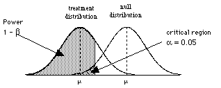
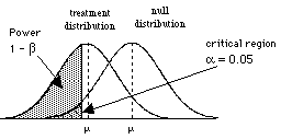
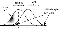
The power of a statistical test is the probability that the test will correctly reject a false null hypothesis. So power is 1 - b.

So, the more "powerful" the test, the more readily it will detect a treatment effect.

So to consider power, we need to consider the situation where H₀ is wrong, that is when there are two populations, the treatment population and the null population

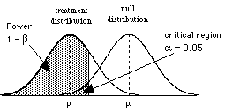
Power is the probability of obtaining sample data in the critical region when the null hypothesis is false.
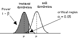
So when there are two populations, the power will be related to how big a difference there is between the two.


	a big difference between the two populationsnotice that the shaded region is large the chance to correctly reject the null hypothesis is good
	a smaller difference between the two populationsnotice that the shaded region is smaller the chance to correctly reject the null hypothesis is not nearly as good

Factors that affect power


1) Increasing a increases power.
2) One-tailed tests have more power than two-tailed tests, given that you have specified the correct tail.


	One-tailed test a = 0.05all of the critical region (a) is on one side of the distribution
	Two-tailed test a = 0.05 because a specific direction is not predicted, the critical region (a) is spread out equally on both sides of the distributionas a result the power is smaller

3) Increasing sample size increases power by reducing the standard error.



	Small n a = 0.05relatively large standard error
	Larger n a = 0.05Smaller standard error as a result the power is greater









Reference: http://psychology.illinoisstate.edu/jccutti/psych240/chpt8.html

Unit -III: Concept of probability

Unit - III: Concept of probability: Probability distribution - normal, poisson, binomial; descriptive

statistics - central tendency, dispersion, skewness and kurtosis.


Sampling: Probability and non-probability

Q 1: What is Probability? Why is it used in psychological research?

Probability:

Suppose there are 25 balls in an urn. 8 among them are blue, 9 are red and 7 are green in color. If now three balls are taken out randomly, what is the likelihood of occurrence that each of the three balls will be of three different colors? The measure of this likelihood of occurrence of an event is called probability. The higher the degree of probability, the more likely the event is to happen, or, in a longer series of samples, the greater the number of times such event is expected to happen. There are a few underlying assumption of probability. These are:

• Equally likely: Elementary events have the same chance of occurrence.
• Mutually Exclusive: If any one of the elementary events occurs then none of the remaining elementary units can occur.
• Elementary events are collectively exhaustive: When taken together they are collectively exhaustive in the sense that no other outcome can occur. Probability is then 1.

Number of ways it can happen

Total number of outcomes

Therefore,

Probability of an event happening =

Example:

There are 5 marbles in a bag: 4 are blue, and 1 is red. What is the probability that a blue marble will be picked?

Number of ways it can happen: 4 (there are 4 blues)

Total number of outcomes: 5 (there are 5 marbles in total)

So the probability =	4/5  = 0.8

Probability in Psychological research:

The concept of probability is relevant to experiments that have somehow uncertain outcomes. There can be situations where despite every effort to maintain fixed (identical conditions) some variations of the result in repeated trials of the experiment are unavoidable. Psychology as a domain of social science deals with individual human being and their behavior, none of which are definite or certain. Consequently psychological research largely involves varied results and findings as because behavior can never be absolutely certain. For example, suppose a child has an IQ of 150. But can we say that the child will definitely score full marks in mathematics? An individual has low trait anxiety. But does it mean that the individual will not be anxious in case of an emergency? So, one of the chief drawbacks of any branch of social scientific research is the presence of several other extraneous variables in addition to the independent and dependent variables. This renders the uncertain nature of psychology. And this is where the concept of probability creeps in. Thus to measure or assess any psychological construct we need the concept of probability in order to make sense out of the distribution of the construct in the larger population. Thus probability is very much required in psychological research.

Q 2: What is Probability Distribution? Describe the characteristics of normal probability distribution.

A probability distribution is a distribution of probabilities of occurrence of scores, events or cases among the classes of the given variable. Probabilities of occurrence of scores can be obtained when the n is large. In such a case the relative frequency (f/n) of scores can be an estimate of their probability of occurrence. In this way a probability distribution may be computed experimentally, using the observed frequencies of scores or events in the data of a test or experiment.

       Theoretically probability distributions, on the contrary, are computed theoretically on the basis of specific mathematical models and laws of probability. They are used widely in predicting probabilities of events and in testing hypothesis experimental hypotheses. Example includes the normal distribution computed on the basis of Gaussian equation. In any probability distribution probabilities are in continuous scale with no real gaps between them. But the scale for events, cases or scores of the variable under consideration may be either continuous or discontinuous. Thus a probability distribution of scores of a discontinuous variable has real gaps in its scale for the scores or cases, and is called a discrete probability distribution. Examples of such distributions are binomial distribution and Poisson distribution. On the other hand a distribution with no real gap in its scale of scores is called a continuous probability distribution such as normal distribution and t- distribution.

Characteristics:

1. The normal probability curve is a bell shaped curve with a single peak at the exact center of the distribution. Thus it is a unimodal distribution.
2. The normal curve is symmetrical about its mean such that the area on the left side of the curve is equal to the right side of the curve.
3. For a normal curve, the arithmetic mean, median and mode lie at the same point i.e. at the centre.
4. The normal probability distribution is asymptotic i.e. the both tails of the curve gets closer and closer to x-axis but touches it.
5. The normal probability distribution is a standardized one i.e. it has a mean of 0 and a standard deviation of 1. Thus for two different standardized normal distributions, any particular observation can be compared by converting the raw score into z-value. Z-value can be obtained by the following formula,

6. The total area under the normal curve is 1. Between the mean and ±3σ of the normal curve, 99.7 % of the total area falls while that between mean and ±2σ is 95.4% and for ±1σ is 68.26%.      

7.   The normal curve follows the Gaussian Equation. The normal distribution is

8.  The normal curve has two inflection points (where the second derivative of f is zero and changes sign), located one standard deviation away from the mean, namely at x = μ − σ and x = μ + σ.

9.   The normal curve has zero skewness as also zero kurtosis. Skewness is the measure of the extent to which a probability distribution of a real-valued random variable "leans" to one side of the mean. It can be positive or negative. On the other hand, kurtosis is any measure of the "peakedness" of the probability distribution of a real-valued random variable. It can be platykurtic (flat) or leptokurtic (too peaked). A normal curve is mesokurtic in nature (no peakedness).

The Poisson Probability Distribution

The Poisson Distribution was developed by the French mathematician Simeon Denis Poisson in 1837.

The Poisson random variable satisfies the following conditions:

1. The number of successes in two disjoint time intervals is independent.
2. The probability of a success during a small time interval is proportional to the entire length of the time interval.

Apart from disjoint time intervals, the Poisson random variable also applies to disjoint regions of space.

Applications

• the number of deaths by horse kicking in the Prussian army (first application)
• birth defects and genetic mutations
• rare diseases (like Leukemia, but not AIDS because it is infectious and so not independent) - especially in legal cases
• car accidents
• traffic flow and ideal gap distance
• number of typing errors on a page
• hairs found in McDonald's hamburgers
• spread of an endangered animal in Africa
• failure of a machine in one month

The probability distribution of a Poisson random variable X representing the number of successes occurring in a given time interval or a specified region of space is given by the formula:

P(X)=​x!​​e​−μ​​μ​x​​​​

where

x=0,1,2,3…
e=2.71828 (but use your calculator's e button)
μ= mean number of successes in the given time interval or region of space

Mean and Variance of Poisson Distribution

If μ is the average number of successes occurring in a given time interval or region in the Poisson distribution, then the mean and the variance of the Poisson distribution are both equal to μ.

E(X) = μ

and

V(X) = σ² = μ

Note: In a Poisson distribution, only one parameter, μ is needed to determine the probability of an event.

Example 1

A life insurance salesman sells on the average 3 life insurance policies per week. Use Poisson's law to calculate the probability that in a given week he will sell

1. Some policies
2. 2 or more policies but less than 5 policies.
3. Assuming that there are 5 working days per week, what is the probability that in a given day he will sell one policy?

Here, μ = 3

(a) "Some policies" means "1 or more policies". We can work this out by finding 1 minus the "zero policies" probability:

P(X > 0) = 1 − P(x₀)

Now P(X)=​x!​​e​−μ​​μ​x​​​​ so P(x​0​​)=​0!​​e​−3​​3​0​​​​=4.9787×10​−2​​

Therefore the probability of 1 or more policies is given by:

Probability=P(X≥0)

=1−P(x​0​​)

=1−4.9787×10​−10​​

=0.95021

(b) The probability of selling 2 or more, but less than 5 policies is:

P(2≤X<5)

=P(x​2​​)+P(x​3​​)+P(x​4​​) 

=​2!​​e​−3​​3​2​​​​+​3!​​e​−3​​3​3​​​​+​4!​​e​−3​​3​4​​​​
=0.61611

(c) Average number of policies sold per day: ​5​​3​​=0.6

So on a given day, P(X)=​1!​​e​−0.6​​(0.6)​1​​​​=0.32929

For reference: http://www.intmath.com/counting-probability/13-poisson-probability-distribution.php